+A Robot Project Data Analysis Documentation

Version: 0.5.0

Edit Time: November 4, 2025

1. Project Background and Content

Business Scenario

The +A Robot Project focuses on the core warehouse sorting scenario (T-sort). Its core business is to realize the full-process automated operations of goods receiving, sorting, and chute discharging via AGV robots (commonly known as "Little Yellow Robots"), serving business lines requiring high-frequency sorting such as e-commerce warehousing and retail supply chains. With the growth of business volume, the traditional operation model has gradually exposed four core pain points:

1. Unclear efficiency bottlenecks: The entire sorting process (task creation → robot scheduling → sorting execution → task closure) lacks quantitative monitoring. Only "overall slowness" can be perceived, and specific bottlenecks (e.g., robot scheduling delays, excessive chute load) cannot be identified.
2. Blind resource allocation: The number of AGV robots is configured based on experience. During peak hours, task backlogs often occur due to insufficient robots; during off-peak hours, resource waste is caused by robot idleness. There is a lack of a scientific prediction model based on workload.
3. Fragmented equipment management: Data on robot status (e.g., charging, faults, mileage) is scattered across different systems and cannot be linked with task execution data (e.g., "whether a faulty robot causes batch delays"). Correlation analysis between equipment health and business efficiency is missing.
4. Cross-team collaboration barriers: Operation, equipment, and IT teams use different data standards, leading to inconsistent data interpretation and low efficiency in problem localization.

Core Project Objectives

To address the above pain points, the project takes "digital-driven full-process sorting efficiency improvement, optimal resource allocation, and early risk warning" as its core objectives, specifically broken down into three aspects:

1. Establish an end-to-end quantitative system: Cover the full dimensions of "task-equipment-system" to enable measurable and traceable sorting efficiency, equipment health, and resource utilization.
2. Deliver scientific decision-making tools: Provide an AGV robot quantity prediction model and optimization plans for resources (charging stations/chutes) to replace experience-based decision-making.
3. Eliminate cross-team data collaboration barriers: Unify data standards and field descriptions to support collaborative analysis among operation, equipment, and IT teams, and shorten problem localization time.

2. Data Linkage Collation

Basic Workflow

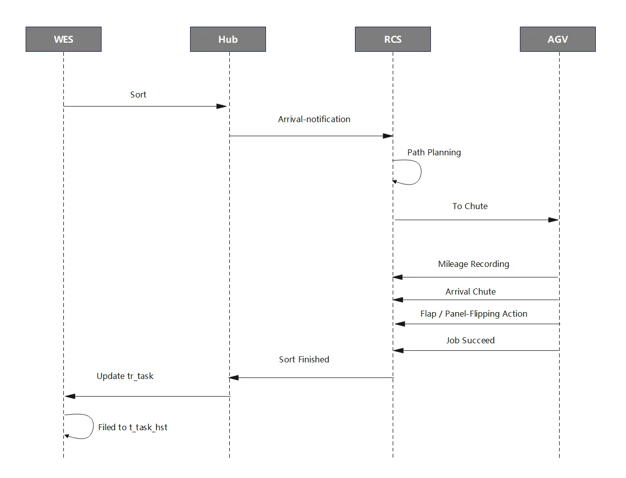
Key Data Closed-Loop (Task Flow)

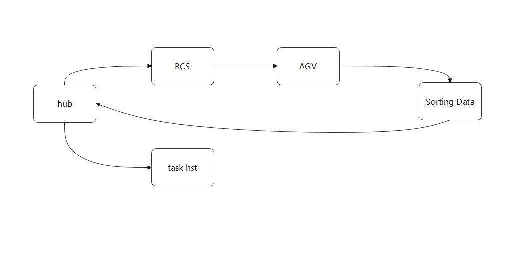
3. Business Themes and Scenario Descriptions

The +A Project mainly focuses on automated sorting, robot operations, and equipment operation monitoring, covering the following business scenarios:

1. Task execution-related Cubes (2 in total): Focus on the "full lifecycle of tasks from creation to completion", including task-level details (Cube_batch_progress_data_details) and batch-level summaries (Cube_batch_progress_data_summary). They cover key fields such as batch_no (batch number), robot_id (robot ID), duration (processing duration), and task_status (task status), supporting quantitative analysis of task efficiency and batch fulfillment.
2. Equipment status-related Cubes (5 in total): Focus on the "full lifecycle status of AGV robots", including charging logs (Cube_wes_db_tsort_charging_log), downtime logs (Cube_wes_db_tsort_downtime_log), driving mileage logs (Cube_wes_db_tsort_odometer_log), power status logs (Cube_wes_db_tsort_power_log), and sorting oper

4. Data Analysis Indicators and Recommendations

Data Analysis Indicators

Batch Task Efficiency

1. Total Tasks, Completed Tasks, Abnormal Tasks: Total Tasks refers to the total number of tasks initiated within a certain period; Completed Tasks refers to the number of successfully executed tasks; Abnormal Tasks refers to the number of tasks that failed to complete normally (e.g., timeout, failure). Together, they reflect the overall execution scale and compliance of tasks.
2. Average/Median Processing Duration, Maximum/Minimum Processing Duration: Average/Median Processing Duration reflects the general level of task time consumption (the median reduces the impact of outliers); Maximum/Minimum Processing Duration reflects extreme fluctuations in time consumption, which is used to evaluate efficiency stability.
3. Robot Utilization Rate (Number of Tasks Assigned per Robot, Average Processing Duration): The number of assigned tasks measures the load intensity of robots; the average processing duration measures the processing efficiency of individual robots. Together, they reflect the adequacy and effectiveness of robot resource utilization.
4. Abnormal Task Ratio (e.g., timeout, failure): The ratio of abnormal tasks to total tasks, which directly reflects the stability of task execution. A higher ratio indicates more prominent process or equipment issues.

Charging Behavior and Energy Consumption

1. Charging Times, Total Charging Duration, Average Charging Duration per Session: Charging Times refers to the total number of charging sessions within a certain period; Total Charging Duration refers to the cumulative charging time; Average Charging Duration per Session refers to the average time consumed per charging session. These are used to analyze whether charging efficiency and frequency are reasonable.
2. Distribution of Charging Peak Periods: Count the proportion of charging times/duration in each time period to identify periods with concentrated charging demand, providing a basis for charging resource scheduling (e.g., charging station allocation).
3. Charging Anomalies (e.g., incomplete charging, charging interruption): Record charging events that do not meet expectations (e.g., stopping before full charge, mid-charge interruption), reflecting health issues of the charging system or batteries.

Downtime and Fault Analysis

1. Total Downtime Times, Total Downtime Duration, Average Downtime Duration per Session: Total Downtime Times and Total Downtime Duration reflect the overall impact scale of downtime; Average Downtime Duration per Session measures the continuous impact of each downtime, which is used to evaluate equipment availability.
2. Distribution of Downtime Causes (e.g., fault, maintenance, unplanned): Count the proportion of downtime by cause (e.g., hardware fault, regular maintenance, sudden unplanned downtime) to identify the main causes of downtime.
3. Downtime High-Frequency Periods and Equipment: Identify time periods (e.g., peak hours) and equipment (e.g., a specific batch of robots) with high downtime frequency to conduct targeted investigations into environmental or individual equipment issues.

Operating Mileage and Utilization Rate

1. Total Driving Mileage, Average Mileage per Equipment: Total Driving Mileage refers to the cumulative driving distance of all equipment, reflecting the overall operation intensity; Average Mileage per Equipment reflects differences in individual equipment usage, which is used to evaluate the balance of equipment load.
2. Equipment Utilization Rate (Operating Duration/Total Available Duration): The ratio of the actual operating duration of equipment to the total available duration (excluding mandatory downtime, etc.), which measures the adequacy of effective work of equipment.
3. Utilization Rate Comparison Between Equipment: Conduct horizontal comparison of utilization rates among different equipment to identify inefficient equipment (low utilization rate) or overloaded equipment (high utilization rate), and optimize resource allocation.

Power Management and Anomaly Monitoring

1. Power On/Off Times, Abnormal Power Interruption Times: Power On/Off Times reflects the frequency of equipment startup and shutdown; Abnormal Power Interruption Times records unplanned power interruption events, which is used to evaluate the stability of the power system.
2. Correlation Analysis Between Power Events and Tasks/Downtime/Charging: Analyze whether power on/off or abnormal power interruption is related to events such as task interruption, equipment downtime, and charging failure, to identify the chain impact of power issues on business.

Sorting Operations and Capacity

1. Total Sorting Volume, Sorting Efficiency (Sorting Volume per Unit Time): Total Sorting Volume refers to the number of sorted items completed within a certain period; Sorting Efficiency refers to the sorting volume per unit time (e.g., per hour), which directly reflects the output capacity of the sorting link.
2. Sorting Anomalies (e.g., cargo jamming, sorting failure): Count abnormal events during the sorting process (e.g., cargo jamming, sorting to the wrong chute), which is used to evaluate the operation stability of sorting equipment.
3. Sorting Peak Periods, Distribution of Sorting Tasks: Identify periods with concentrated sorting volume and task types (e.g., specific chutes/areas) to provide a basis for dynamic adjustment of sorting resources (e.g., robot scheduling, chute maintenance).

Analysis Approach Recommendations

1. Multi-dimensional comparison: Compare various indicators by dimensions such as time (daily/weekly/monthly), equipment, robot, and team to identify bottlenecks and anomalies.
2. Trend analysis: Focus on the changing trends of key indicators (e.g., task efficiency, downtime duration, charging times) over time to identify potential optimization space.
3. Anomaly tracking: Conduct detailed tracking of abnormal tasks, downtime, and charging anomalies to locate problematic equipment or high-frequency periods.
4. Correlation analysis: Analyze correlations such as downtime vs. charging, and sorting anomalies vs. equipment status to support operation and maintenance decisions.
5. Capacity evaluation: Combine sorting logs and task logs to evaluate the gap between actual capacity and theoretical capacity.

5 Visualization Scheme Examples

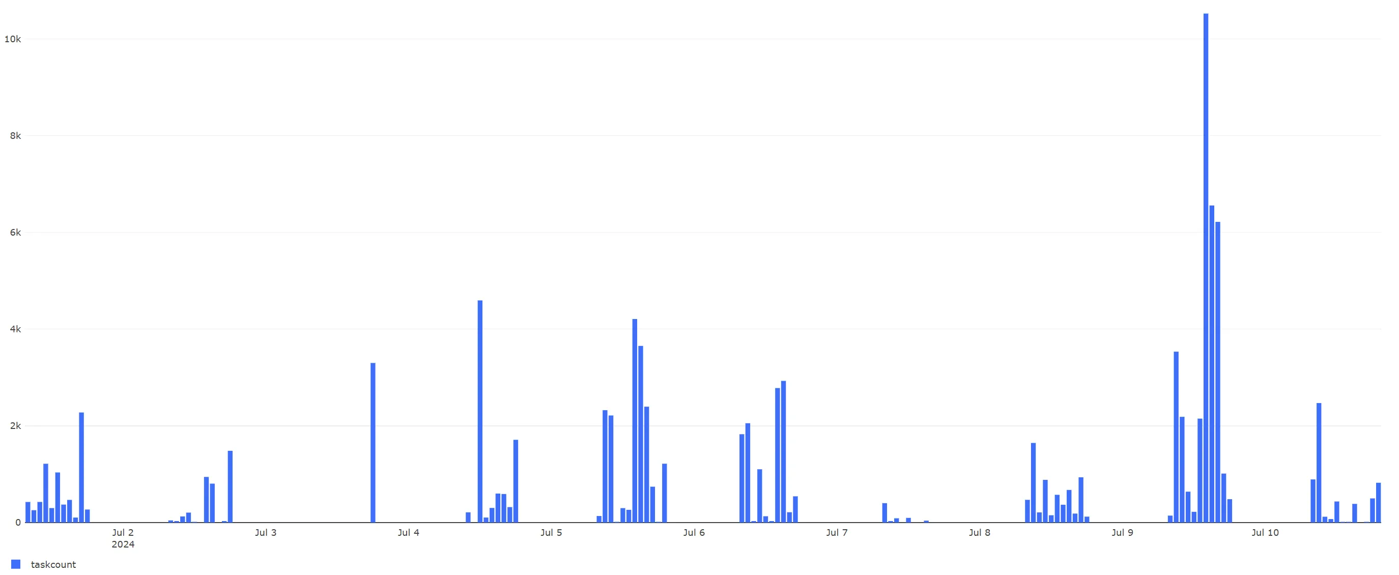
1. Overall Throughput Analysis (Cube_batch_progress_data_details)
   • Indicator: Total tasks per hour (units/hour), i.e., the number of tasks completed per hour, used to reflect the overall operation capacity.
   • Dimension: hourTime (hour, formatted as YYYY-MM-DD HH24:00:00)
   • Visualization: Bar Chart or Line Chart, showing the changing trend of tasks per hour over time to intuitively reflect capacity fluctuations in different periods.

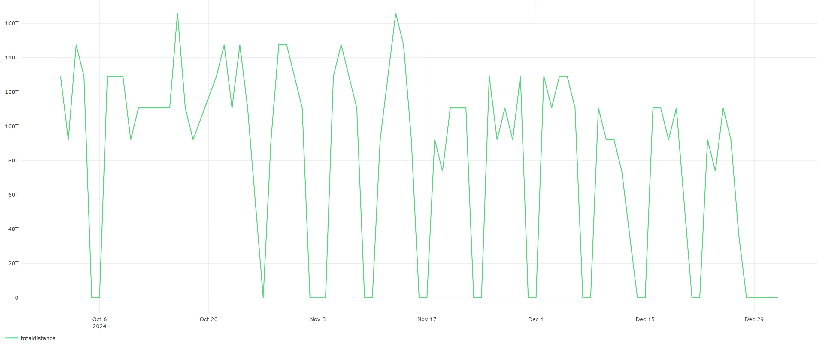
2. Robot Operating Mileage Trend (Cube_wes_db_tsort_odometer_log)
   • Indicator: Daily total driving mileage, i.e., the sum of left-wheel and right-wheel driving distances of all robots on a given day.
   • Dimension: runDate (date, formatted as YYYY-MM-DD)
   • Visualization: Line Chart, showing the changing trend of daily total driving mileage to reflect the time distribution of the overall operation intensity of robots.

3. Equipment Downtime Duration Distribution (Cube_wes_db_tsort_downtime_log)
   • Indicator: Total downtime duration by type (unit: seconds), i.e., the sum of durations of all records under the same downtime type.
   • Dimension: downtimeType (downtime type)
   • Visualization: Pie Chart or Stacked Bar Chart, showing the proportional relationship of downtime duration by type to clarify the impact degree of major downtime causes.

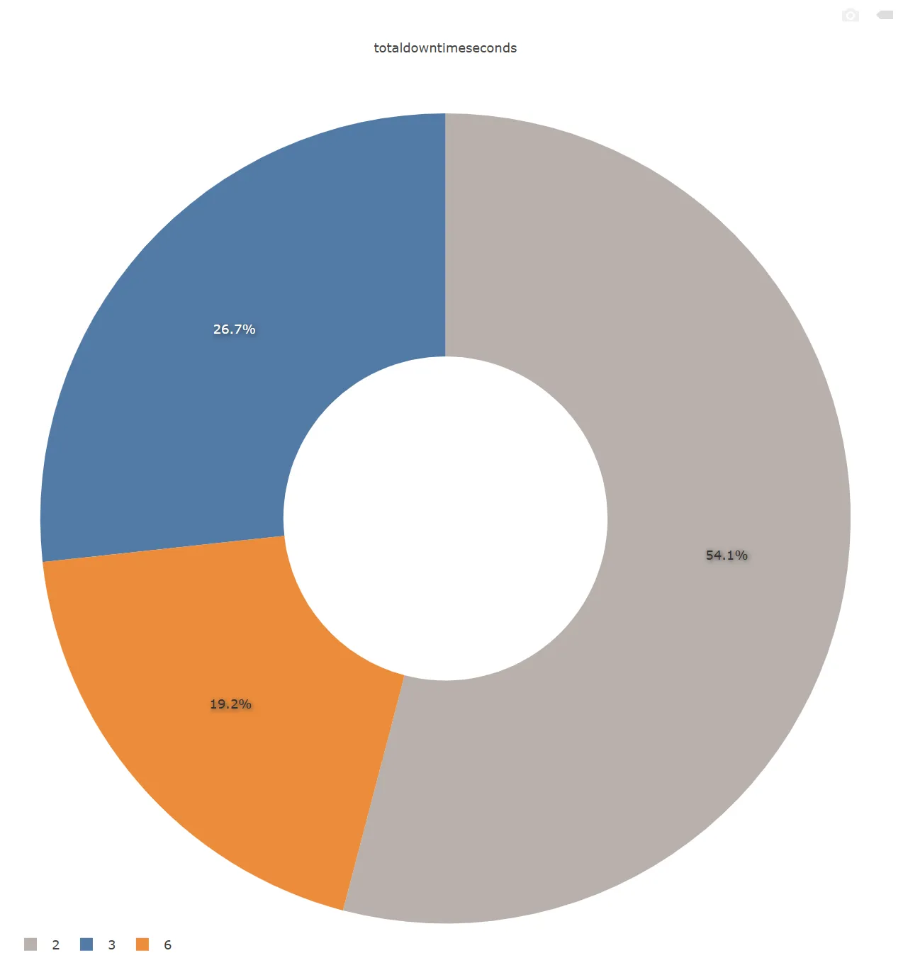
Check URL to view the dashboard for the three charts above： http://bi-dashboard.item.com/public/dashboards/WFyVMScMUbDoITdqdqUlHlGiaOMOLSBsSjtkuEze?org_slug=default

4. Overall Visualization Case Display

The following analyses are all based on Cube_batch_progress_data_details, focusing on the 2024 task volume (counted by batch_detail_no, representing the number of task units). They cover five dimensions—"total volume, daily average, peak value, daily trend, and robot contribution ratio"—to fully present the annual operation scale, fluctuation rules, and robot load distribution, providing data support for capacity evaluation and resource scheduling.

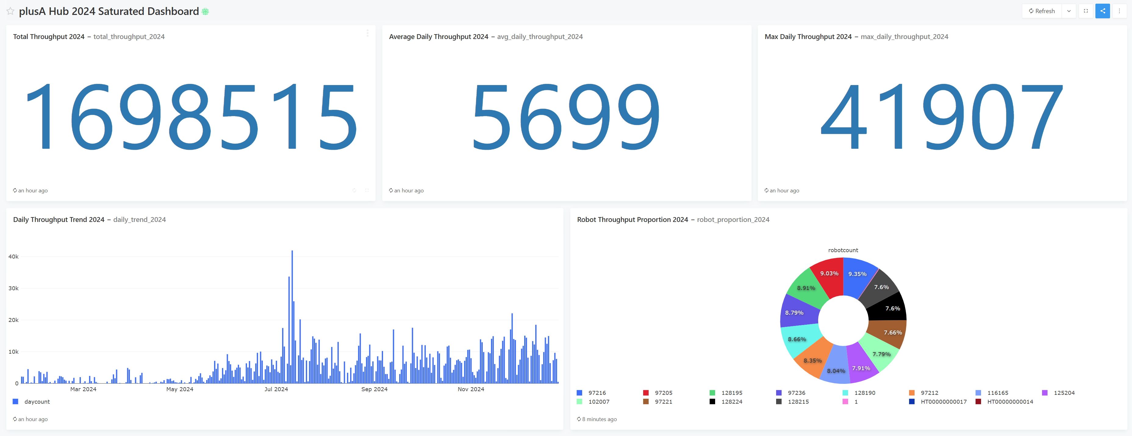
Check URL for Dashboard：

http://bi-dashboard.item.com/public/dashboards/jnRM78NVPKZh2R0AzsE4Ymv5gXOr3IqOMuB78ZGc?org_slug=default

1. 2024 Total Volume Statistics (Cube_batch_progress_data_details)
   • Indicator: 2024 total task units, i.e., the cumulative number of all batch_detail_no in 2024, reflecting the overall annual operation scale.
   • Dimension: Full year 2024 (time range limited to 2024-01-01 to 2024-12-31)
   • Visualization: Number Card, intuitively displaying the total annual units, which can be supplemented with comparison labels with other years.
2. 2024 Daily Average Volume Statistics (Cube_batch_progress_data_details)
   • Indicator: 2024 daily average task units, i.e., the average of daily task units in 2024, reflecting the average daily load of daily operations.
   • Dimension: Full year 2024 (calculated based on daily statistics results)
   • Visualization: Number Card, which can simultaneously display the correlation between "total annual units" and "daily average units" to help understand the relationship between the overall and daily levels.
3. 2024 Maximum Daily Volume and Corresponding Date (Cube_batch_progress_data_details)
   • Indicator: 2024 maximum daily task units and the corresponding date, reflecting the annual peak operation load and its occurrence time.
   • Dimension: Specific date (a day in 2024, formatted as YYYY-MM-DD)
   • Visualization: Number Card + Text Annotation (e.g., "Maximum Daily Volume: X units (2024-XX-XX)"), or highlight the peak date in a Bar Chart to clearly locate the volume peak.
4. 2024 Daily Volume Trend (Cube_batch_progress_data_details)
   • Indicator: 2024 daily task units, reflecting the daily fluctuation rules of annual volume (e.g., seasonality, weekly cycle, sudden peaks).
   • Dimension: workDay (daily in 2024, formatted as YYYY-MM-DD)
   • Visualization: Line Chart or Bar Chart, with the horizontal axis as the date and the vertical axis as daily units. It allows intuitive observation of the upward/downward trend of annual volume, the distribution of peaks and troughs, and periodic characteristics.
5. 2024 Task Volume Ratio by Robot (robot_id) (Cube_batch_progress_data_details)
   • Indicator: 2024 task units of each robot and their percentage of the total volume, reflecting the load of different robots and their contribution ratio to the overall capacity.
   • Dimension: robotId (unique robot identifier)
   • Visualization: Pie Chart (showing ratio distribution) or Bar Chart (sorted by task units in descending order, with ratio labels), which can quickly identify high-load robots and the balance of resource allocation.

6. Advanced Analysis and Prediction Approach

To predict the number of "Little Yellow Robots" (AGV robots) required based on workload, the core is to establish a matching model between "workload demand" and "robot effective capacity". This model should combine historical data, task characteristics, robot performance, and scenario constraints. The approach is divided into 6 key steps:

Step 1: Define Quantitative Indicators for "Workload"

First, "workload" must be converted into computable quantitative indicators to avoid ambiguity. The core indicators include:

1. Total Tasks (T):
   The total number of tasks to be completed within a unit time (e.g., daily average sorting tasks, total batches).

   • Source: Historical task data (e.g., summary of task_count from dwd_batch_progress_data_summary) and business demand forecasts (e.g., estimated increment during promotion periods).
   • Note: Distinguish between "effective tasks" (requiring robot execution) and "invalid tasks" (e.g., manually intervened tasks).

2. Average Processing Time per Task (t):
   The average time from task assignment to completion for a single task (unit: hour/minute).

   • Calculation: Based on the duration of historical tasks (e.g., end_time - start_time from dwd_batch_progress_data_details), excluding outliers (e.g., timeout tasks, empty tasks).
   • Segmentation: The processing time of different task types (e.g., task_type) may vary significantly (e.g., "urgent sorting" vs. "regular sorting"), so t should be calculated separately for each type.

Step 2: Determine "Time Window" and "Work Mode"

The time dimension for prediction (e.g., daily, hourly, peak periods) and the robot work mode must be clarified to avoid deviations in capacity calculation:

1. Time Window (W):

   • Basic window: e.g., "daily working hours" (e.g., 8 hours, 12 hours).
   • Peak window: Calculate the workload during peak periods (e.g., 9:00-11:00 daily) separately to avoid resource shortages caused by short-term congestion.

2. Work Mode Constraints:

   • Continuous operation or shift-based operation? (e.g., two-shift system: morning shift 8:00-20:00, night shift 20:00-8:00).
   • Mandatory downtime for maintenance? (e.g., 2:00-4:00 daily).

Step 3: Calculate "Effective Capacity per Robot"

The actual capacity of a robot is not simply "Time Window × 100% Utilization Rate"; non-working time (charging, faults, idleness, etc.) must be deducted. The core parameters include:

1. Effective Operating Duration per Robot per Unit Time (E):

   • Formula: E = Time Window (W) × Effective Utilization Rate (U)

   • Effective Utilization Rate (U): The ratio of the actual operating time of the robot to the total time, which needs to deduct:

     • Charging time ratio (C): e.g., if the daily average charging time is 2 hours, accounting for 16.7% of the 12-hour work window, then C = 16.7%.
     • Fault/downtime ratio (D): e.g., if the daily average fault time is 0.5 hours, accounting for 4.2%, then D = 4.2%.
     • Idle time ratio (I): The waiting time between tasks, e.g., 1 hour daily on average, accounting for 8.3%, then I = 8.3%.

   • Example: U = 1 - C - D - I = 1 - 16.7% - 4.2% - 8.3% = 70.8%; if W = 12 hours, then E = 12 × 70.8% ≈ 8.5 hours.

2. Task Processing Volume per Robot per Unit Time (P):

   • Formula: P = Effective Operating Duration (E) / Average Processing Time per Task (t)
   • Example: If E = 8.5 hours and t = 5 minutes/task (i.e., 0.083 hours/task), then P = 8.5 / 0.083 ≈ 102 tasks/day.

Step 4: Establish Basic Prediction Model: Theoretical Required Quantity

Calculate the theoretical minimum quantity based on "total workload" and "per-robot capacity":

1. Basic Formula:
   Theoretical Number of Robots (N_base) = Total Tasks (T) / Task Processing Volume per Robot per Unit Time (P)

   • Example: If the daily average total tasks T = 10,000 tasks and per-robot P = 102 tasks/day, then N_base = 10,000 / 102 ≈ 98 units.

2. Segmentation by Task Type:
   If there are multiple task types (e.g., Type A, B, C) with significant differences in processing time, calculate separately and then summarize:

   • N_A = T_A / P_A
   • N_B = T_B / P_B
   • N_total_base = N_A + N_B + ...

Step 5: Dynamic Adjustment: Incorporate Peak and Redundancy Coefficients

In actual scenarios, workload fluctuations, sudden anomalies, and other risks must be considered to adjust the theoretical quantity:

1. Peak Coefficient (K1):

   • Used to cope with short-term workload surges (e.g., promotion days, morning/evening peaks).
   • Calculation: K1 = Historical Maximum Hourly Task Volume / Historical Average Hourly Task Volume
     (e.g., if the peak-hour task volume is 1.5 times the average, then K1 = 1.5)

2. Redundancy Coefficient (K2):

   • Used to cope with uncontrollable factors such as temporary robot faults, charging queues, and task assignment deviations.
   • Empirical value: Usually 1.1-1.3 (e.g., 10%-30% redundancy), with a higher value when equipment stability is poor.

3. Adjusted Formula:
   Actual Required Number of Robots (N_actual) = N_base × K1 × K2

   • Example: N_base = 98 units, K1 = 1.5, K2 = 1.2, then N_actual = 98 × 1.5 × 1.2 ≈ 177 units.

Step 6: Verification and Iteration: Calibrate the Model with Historical Data

The prediction model must be verified with historical data to avoid discrepancies between theory and practice:

1. Backtesting:

   • Select historical data from the past 3 months, use the model to infer the "theoretical required quantity", compare it with the actual number of robots used, and calculate the deviation rate:
     Deviation Rate = |Model Value - Actual Value| / Actual Value
   • If the deviation rate > 20%, adjust parameters (e.g., recalculate the effective utilization rate U, average processing time per task t).

2. Scenario-Specific Fine-Tuning:

   • New warehouses/new robots: Due to insufficient data, refer to K1 and K2 of similar scenarios, use a higher redundancy coefficient (e.g., 1.3) initially, and gradually lower it based on actual operation data.
   • Seasonal fluctuations: During periods such as e-commerce promotions, K1 needs to be temporarily increased (e.g., 2.0) to avoid resource shortages.

Summary: Core Logic Chain

Workload (Total Tasks × Average Processing Time per Task) → Effective Capacity per Robot (Time Window × Utilization Rate ÷ Average Processing Time per Task) → Theoretical Quantity → Incorporate Peak/Redundancy Coefficients → Actual Required Quantity.

This approach enables the transition from "passive response" to "proactive planning", avoiding both resource waste (robot idleness) and task delays caused by insufficient quantities.